Smith-Wilson yield curves
Let’s start this journey with the most basic, yet most important “parameters” of any solvency 2 calculations : the risk-free interest rate. EIOPA, the european insurance and occupational pensions authority uses the Smith-Wilson model to publish the relevant risk free interest rate term structures, also called the RFR.
According to article 77 of the Solvency 2 directive, the best estimate of technical provisions shall correspond to the probability-weighted average of future cash-flows, taking account of the time value of money (expected present value of future cash-flows), using the relevant risk-free interest rate term structure. \[Best\_Estimate=\mathbb{E}\left[\sum_{t≥0}Cashflow_t \cdot P(t)\right]\] where \(P(t)\) is the price of a zero-coupon bond of maturity \(t\) priced with the relevant risk free interest rate term structures as set out by EIOPA.
Smith-Wilson model
This article is based on the work of the Financial Supervisory Authority of Norway, so feel free to check it out here.
We assume that we have N interest related financial instruments as input and J different dates at which a cash payment has to be made on behalf of at least one of these instruments.
- We need the market prices \(m_i\) of the instruments \(i\) at valuation date, for \(i \in [ 0,N ]\).
- cash payment dates \(u_1,u_2,u_3,u_4, ...,u_J\) for the instruments,
- The cash-flows \(c_{i,1},c_{i,2},c_{i,3},...,c_{i,J}\).
The general pricing function at valuing time proposed by Smith and Wilson is :
\[P(t)=e^{-ufr \cdot t}+\sum_{i=1}^N \zeta_i \cdot \left( \sum_{j=1}^J c_{i,j}\cdot W(t,u_j)\right)\]
where
\[\sum_{j=1}^J c_{i,j}\cdot W(t,u_j)=:K_i(t) \] is called the kernel functions. \(W(t,u_j)\) is defined like this :
\[W(t,u_j)=e^{-ufr\cdot (t+u_j)}\cdot \left[ \alpha\cdot \min(t,u_j) -0.5\cdot e^{-\alpha\cdot \max(t,u_j)}\cdot(e^{\alpha\cdot \min(t,u_j)}-e^{-\alpha\cdot\min(t,u_j)}) \right]\] We can clearly identify 2 different parameters that are :
- \(ufr\) : the continously compounded ultimate forward rate, to be chosen outside the model. In the Solvency 2 framework, this rate is set to \(ln(1+0.042)=0.04114194\).
- \(\alpha\) : convergence speed rate (how fast will the rates converge to the ufr?) to be chosen outside the model. Let’s assume for the moment that this value is \(0.10\).
The market price of a risk-free bond \(i\) is basically the sum of its discounted coupons, i.e.
\[m_i = \sum_{j=1}^Jc_{i,j}\cdot P(u_j)\] As you may have noticed, if we had the prices of all zero coupon bonds \(P(u_j)\) then the work here would be over and we wouldn’t have started this article in the first place. But we want to find a way to assess these prices and we will do this by inputing the general Smith Wilson pricing function in the formula above :
\[ \begin{aligned} m_i &= \sum_{j=1}^Jc_{i,j}\cdot P(u_j) \\ &= \sum_{j=1}^Jc_{i,j}\cdot \left[ e^{-ufr \cdot u_j}+\sum_{l=1}^N \zeta_l \cdot \left( \sum_{k=1}^J c_{i,k}\cdot W(u_j,u_k)\right) \right] \\ &= \sum_{j=1}^Jc_{i,j}\cdot e^{-ufr \cdot u_j}+ \left[ \sum_{l=1}^N \zeta_l \cdot \left( \sum_{k=1}^J c_{i,k}\cdot \sum_{j=1}^J \{c_{i,j}\cdot W(u_j,u_k)\}\right) \right] \\ &= \sum_{j=1}^Jc_{i,j}\cdot e^{-ufr \cdot u_j}+ \left[ \sum_{l=1}^N \left( \sum_{k=1}^J \left\{\sum_{j=1}^J c_{i,j}\cdot W(u_j,u_k)\right\}\cdot c_{i,k}\right) \cdot \zeta_l \right] \\ \end{aligned} \] We thus have here the full system in vectorial notation
\[ \begin{aligned} m &= C\cdot p \\ &= C\cdot \mu+(CWC^T)\zeta \\ &= M(N\times N) \cdot M(N \times 1)\\ &+ \left[M(N\times J)\cdot M(J \times J)\cdot M(J \times N)\right]\cdot M(N\times 1)\\ &= M(N\times 1) \end{aligned} \] with \(\mu=(e^{-ufr\cdot u_1},e^{-ufr\cdot u_2},e^{-ufr\cdot u_3},...,e^{-ufr\cdot u_J})^T\). We can also check that this system makes sense by checking the dimensions of the matrices
\[ \begin{aligned} C\cdot p &= C\cdot \mu+(CWC^T)\zeta \\ M(N\times N) \cdot M(N \times 1) &= M(N\times N) \cdot M(N \times 1) \\ &+\left[M(N\times J)\cdot M(J \times J)\cdot M(J \times N)\right]\cdot M(N\times 1)\\ M(N\times 1) &= M(N\times 1) \end{aligned} \] We therefore have all the ingredients to calculate \(\zeta = (CWC^T)^{-1}(m-C\cdot \mu)\).
Example
Let’s consider 4(=N) at par bonds with maturities 1,2,3,5 and coupons :
##   Maturity Coupon Price
## 1        1  0.010     1
## 2        2  0.020     1
## 3        3  0.026     1
## 4        5  0.034     1
So \(\max(Maturity)=5\) and thus \(u_1=1,...,u_4=4,u_5=5\) even though we only have 4 bonds. We can also construct the cash-flow matrix :
##    Bond_1 Bond_2 Bond_3 Bond_4
## u1   1.01   0.02  0.026  0.034
## u2   0.00   1.02  0.026  0.034
## u3   0.00   0.00  1.026  0.034
## u4   0.00   0.00  0.000  0.034
## u5   0.00   0.00  0.000  1.034
The W matrix
Let’s recall the formula here \[W(t,u_j)=e^{-ufr\cdot (t+u_j)}\cdot \left[ \alpha\cdot \min(t,u_j) -0.5\cdot e^{-\alpha\cdot \max(t,u_j)}\cdot(e^{\alpha\cdot \min(t,u_j)}-e^{-\alpha\cdot\min(t,u_j)}) \right]\]
In this section, we will see how easily we can build this \(W\) matrix. First thing we can notice is that \(W(t,u_j)=W(u_j,t)\), which means that \(W\) will be a symmetric matrix in this case. We could build \(W\) by using 2 for loops, i.e. for t = 1:T and for uj=1:J etc. but there’s a much nicer way of building this W matrix.
Let t be represented by the columns of our matrix and \(u_j\) the rows, in that case, we can build two matrices T.mat (\(=t\)) and U (\(=u_j\))
print(T.mat)## [,1] [,2] [,3] [,4] [,5]
## [1,] 1 2 3 4 5
## [2,] 1 2 3 4 5
## [3,] 1 2 3 4 5
## [4,] 1 2 3 4 5
## [5,] 1 2 3 4 5print(U)## [,1] [,2] [,3] [,4] [,5]
## [1,] 1 1 1 1 1
## [2,] 2 2 2 2 2
## [3,] 3 3 3 3 3
## [4,] 4 4 4 4 4
## [5,] 5 5 5 5 5Now that we have T.mat and U, we can compute \(t+u_j\), \(\min(t,u_j)\) and \(\max(t,u_j)\)
print(T.mat+U)## [,1] [,2] [,3] [,4] [,5]
## [1,] 2 3 4 5 6
## [2,] 3 4 5 6 7
## [3,] 4 5 6 7 8
## [4,] 5 6 7 8 9
## [5,] 6 7 8 9 10min_tuj<-pmin(T.mat,U)
max_tuj<-pmax(T.mat,U)
print(min_tuj)## [,1] [,2] [,3] [,4] [,5]
## [1,] 1 1 1 1 1
## [2,] 1 2 2 2 2
## [3,] 1 2 3 3 3
## [4,] 1 2 3 4 4
## [5,] 1 2 3 4 5print(max_tuj)## [,1] [,2] [,3] [,4] [,5]
## [1,] 1 2 3 4 5
## [2,] 2 2 3 4 5
## [3,] 3 3 3 4 5
## [4,] 4 4 4 4 5
## [5,] 5 5 5 5 5Let’s recall the formula of \(\zeta\) which is \(\zeta = (CWC^T)^{-1}(m-C\cdot \mu)\). We now have \(C\),\(W\) and \(\mu\).
ufr<-log(1+0.042)
a<-0.1

m<-input$Price
W<-exp(-ufr*(T.mat+U))*(a*min_tuj-0.5*exp(-a*max_tuj)*(exp(a*min_tuj)-exp(-a*min_tuj)))

mu<-exp(-ufr*(1:J))

zeta<-solve(t(C)%*%W%*%C)%*%(m-t(C)%*%mu)
print(W)
## [,1] [,2] [,3] [,4] [,5]
## [1,] 0.00862561 0.01590149 0.02188057 0.02674724 0.03066104
## [2,] 0.01590149 0.02982485 0.04139268 0.05081327 0.05839446
## [3,] 0.02188057 0.04139268 0.05813003 0.07188306 0.08296295
## [4,] 0.02674724 0.05081327 0.07188306 0.08970176 0.10417950
## [5,] 0.03066104 0.05839446 0.08296295 0.10417950 0.12189849print(mu)## [1] 0.9596929 0.9210105 0.8838872 0.8482603 0.8140694print(zeta)## [,1]
## [1,] 57.790688
## [2,] -33.507208
## [3,] 11.396473
## [4,] -5.466968Now that we have our zeta parameters we can build the whole curve, even for the maturities over \(J\). For this, we will need to extend \(W\), say we want to get the curve up to 50 years (\(=K\)).
K<-50
T.mat<-t(matrix(1:J,J,K))
U<-(matrix(1:K,K,J))

min_tuj<-pmin(T.mat,U)
max_tuj<-pmax(T.mat,U)


W<-exp(-ufr*(T.mat+U))*(a*min_tuj-0.5*exp(-a*max_tuj)*(exp(a*min_tuj)-exp(-a*min_tuj)))
Let’s look at the shape of this extended W function :

As we can see, the values of \(W(t,u_j)\) decrease as t increases, its effect on the final price \(P(t)\) becomes less and less relevant.
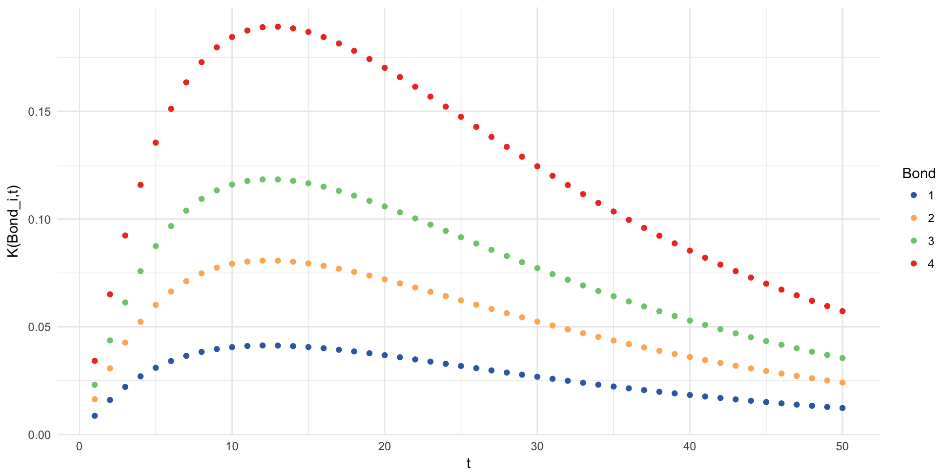
Just as stated above, as the effect of \(W(t,u_j)\) decreases, the importance of the kernel functions \(K_i(t) = \sum_{j=1}^J c_{i,j}\cdot W(t,u_j)\) also decreases.
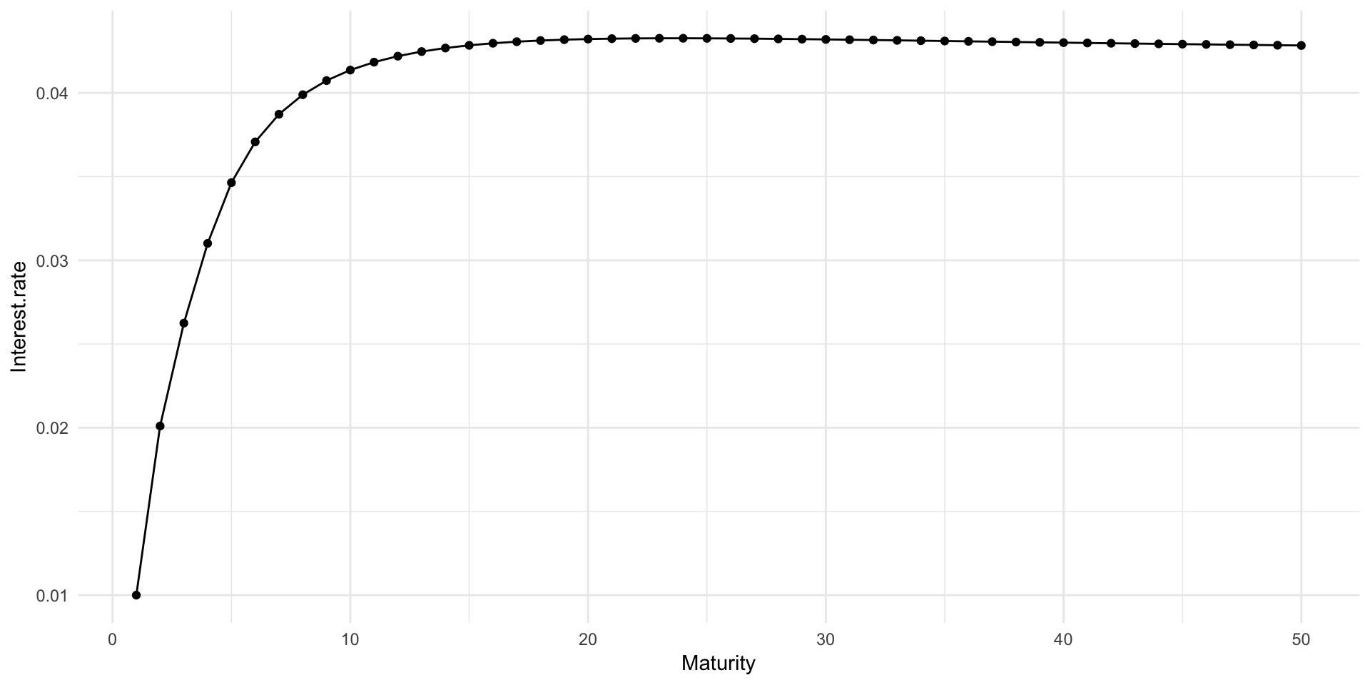
Let’s split the function \[P(t)=\underbrace{e^{-ufr \cdot t}}_{A}+\underbrace{\sum_{i=1}^N \zeta_i \cdot \left( \sum_{j=1}^J c_{i,j}\cdot W(t,u_j)\right)}_{B}\] into two parts and plot their values on a graph.
We see that the values of \(B\) are almost negligible after a certain maturity \(t\) and thus \(P(t)\) converges to \(A\). The interest rates converge therefore to the planned ultimate forward rate of \(4.2%\) annually compounded.
Impact of alpha
Now let’s wrap this up neatly into a function and plot the impact of different alphas.
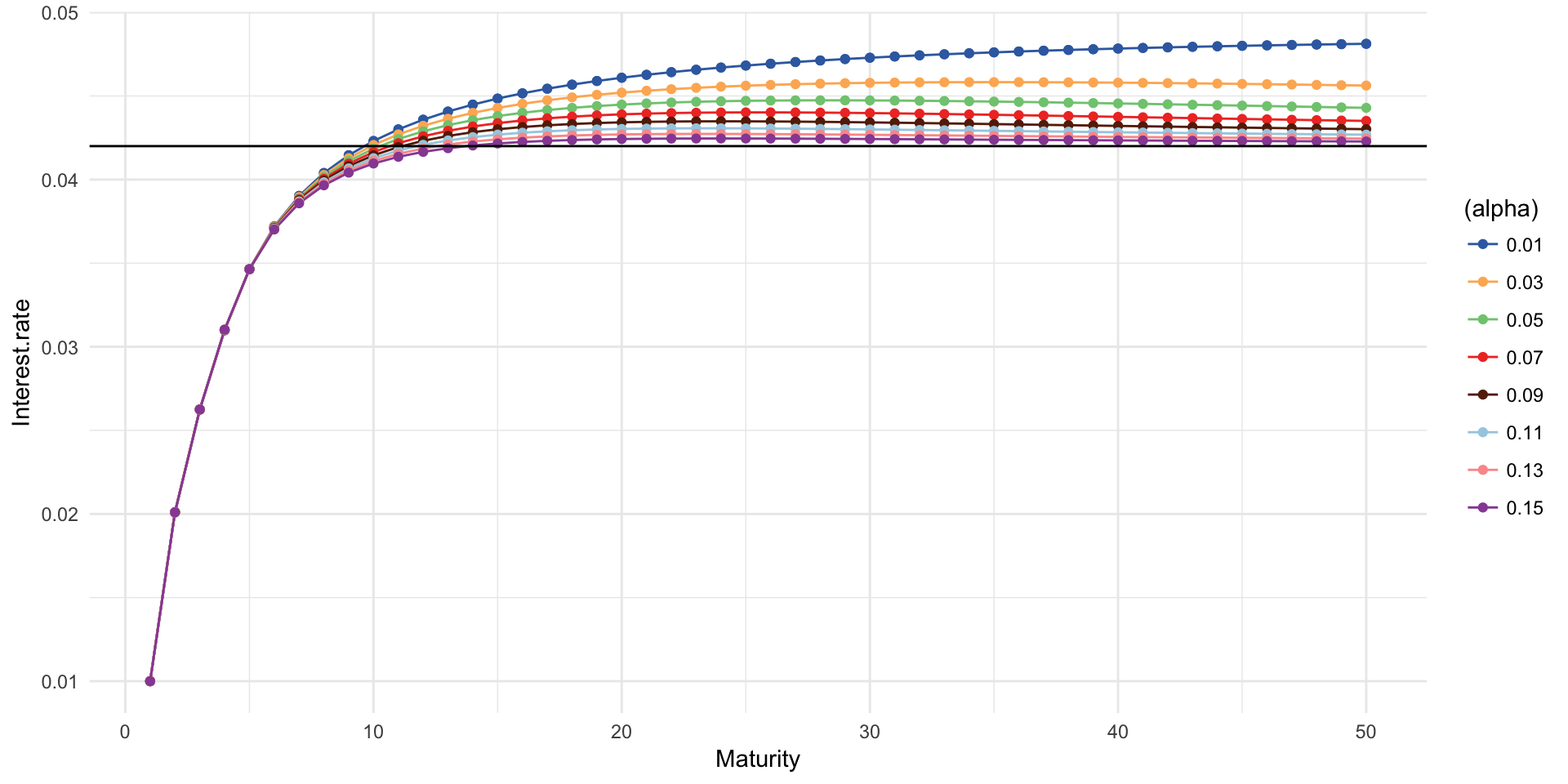
Just as expected, \(\alpha\) changes the speed at which the rates converge to the annually compounded ultimate forward rate. In our example, rates take more time to converge when \(\alpha<0.10\).
Impact of the ultimate forward rate
For this section, let’s assume that we have these dummy risk-free bonds and plot the corresponding interest rates according to different ufr.
##    Maturity   Coupon Price
## 1         2 -0.00696     1
## 2         3 -0.00571     1
## 3         4 -0.00425     1
## 4         5 -0.00300     1
## 5         6 -0.00158     1
## 6         7 -0.00036     1
## 7         8  0.00076     1
## 8         9  0.00224     1
## 9        10  0.00305     1
## 10       15  0.00688     1
## 11       20  0.00854     1
We can see that the curves are relatively similar up to the last liquid point of 20 years thanks to the effects of the kernel functions \(=B\) and have a little bump when the ufr is significantly higher than the zero coupon rate of the highest maturity (e.g. 5% compared to 0.88%).
Thanks for reading!
END
Credits :
