Quantify life ?
Life insurance
Classical life insurance is all about interest rate and mortality. Let’s take for example a whole life insurance contract which is basically a contract with a payment at the end of the year of death of the insured to the beneficiary, a good classical life insurance contract.
In order to model this, we need to
- model the future lifetime
- model the interest rates in order to discount this payment
Life actuaries use fancy notations to express their “things”, so in order to understand what’s going on let me list here some simple notations :
- \(x\) defines the age of a person
- \(l_x\) defines the number of persons still alive at age x
- TH00_02 (male) and TF00_02 (female) are two french life tables that were introduced in 2007.
From life tables to future lifetime
Fortunately there exists a lovely life insurance r package lifecontingencies with a bunch of useful datasets and actuarial functions. So without further ado let’s take a look into this :
data("demoFrance")
demoFrance<-rbind(demoFrance,c(113,0,0,0,0)) # this will be needed later
french.lifetables<-melt(demoFrance,id.vars = "age")
names(french.lifetables)<-c("age","Life.table","lx")

ggplot(french.lifetables[french.lifetables$Life.table%in%c("TH00_02","TF00_02"),],
       aes(x=age,y=lx,color=Life.table))+
  geom_line()+
  theme_minimal()+
  xlab("x = age")+
  scale_colour_manual(values=colorpal)+
  theme(legend.position="bottom")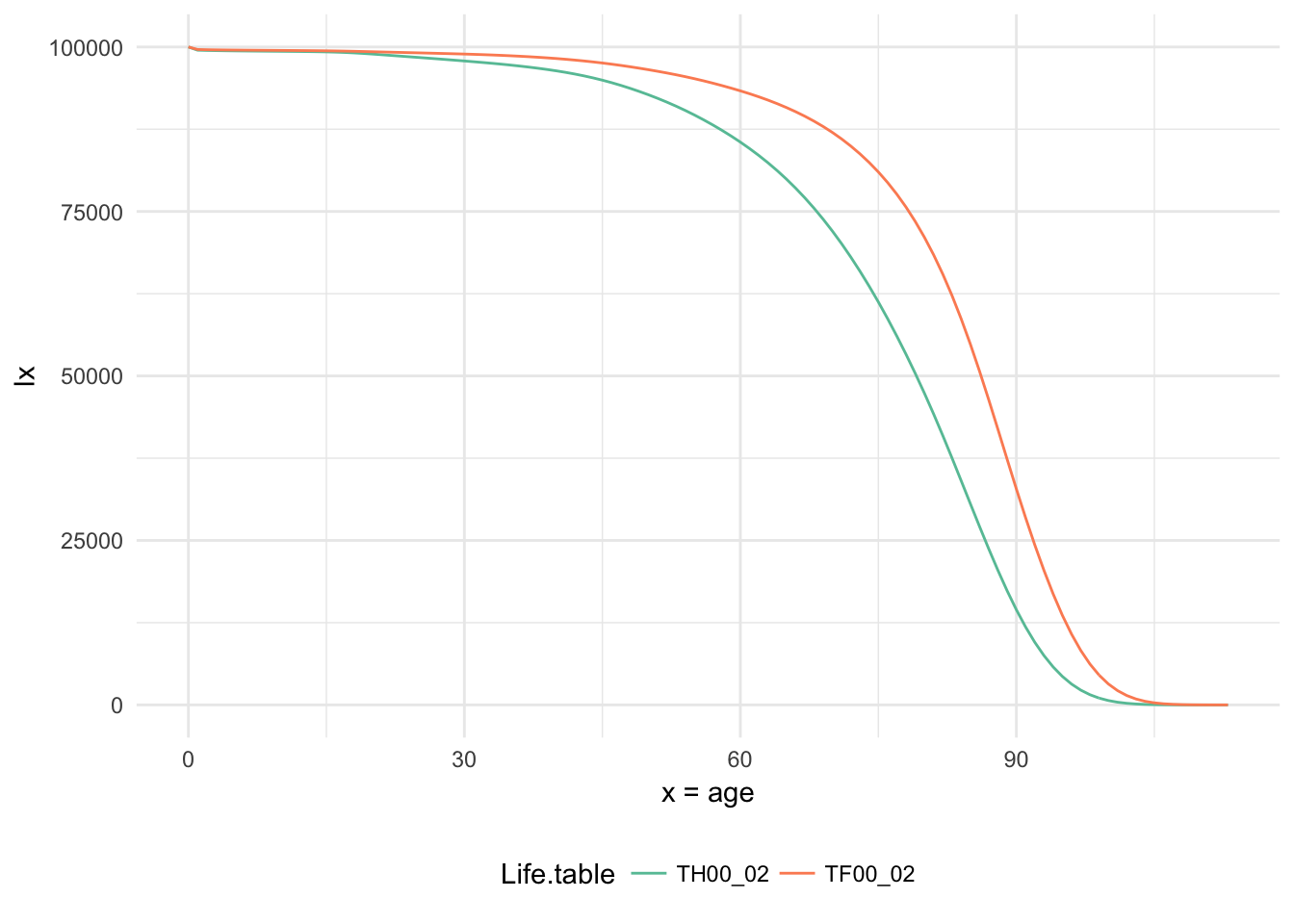
The curves here \((l_x)\) which are once again the number of person still alive at the age of \(x\) have an impressive rollercoast descent starting at around 50 for men and around 60 for women. So this confirms the sayings that women live longer than men. We can summarise the information of these curves into a single indicator which is the life expectancy at birth and compare the longevity of different groups of people. So let \(T(x)\) be the random variable defining the future lifetime or the age at death. Its mean value is called the life expectancy :
\[ \mathbb{E}(T(x))=\sum_{x=0}^\infty x\cdot \mathbb{P}[T=x] \] with \(\mathbb{P}[T=x]=\mathbb{P}[\text{survive from birth until $x$ and then die}] = \frac{l_x}{l_0} \cdot \frac{l_x-l_{x+1}}{l_x}\), for example the probability to die at the age of 60 given that the person is a baby is \[ \begin{aligned} \mathbb{P}[T=60|x_0=0]&=\frac{\textit{#survivors_60_years_later}}{\textit{#survivors_at_the_beginning}}\cdot \frac{\textit{#deceased_at_the_age_of_60}}{\textit{#survivors_60_years_later}}\\ \mathbb{P}[T=60|x_0=0]&=\frac{l_{60}}{l_{0}}\cdot \frac{l_{60}-l_{61}}{l_{60}}=\frac{l_{60}-l_{61}}{l_0}\\ \end{aligned} \] so basically, \(\mathbb{P}[T=x|x_0]=\frac{l_{x}-l_{x+1}}{l_{x_0}}\). We can also check that these probabilities make sense by summing them up on \(x\) :
\[ \begin{aligned} \sum_{x=x_0}^\infty \mathbb{P}[T=x|x_0] = \mathbb{P}[T<\infty|x_0] &= \sum_{x=x_0}^\infty \left[\frac{l_{x}-l_{x+1}}{l_{x_0}}\right]\\ &= \dfrac{l_{x_0}-l_{x_0+1}}{l_{x_0}}+\dfrac{l_{x_0+1}-l_{x_0+2}}{l_{x_0}}+\dfrac{l_{x_0+2}-l_{x_0+3}}{l_{x_0}}+...\\ &\rightarrow \dfrac{l_{x_0}-\overbrace{l_{\infty}}^{\rightarrow 0}}{l_{x_0}} \rightarrow 1 \end{aligned} \]
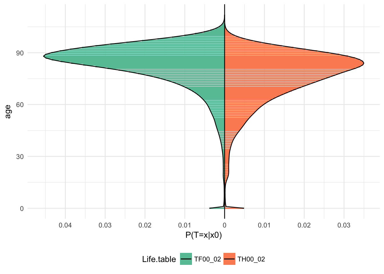
There’s a little bump at the beginning where babies and children up to 4 are more fragile and thus have a higher probability to die.
So, if we come back to our life expectancy at birth:
e_x<-(PT %>% group_by(Life.table) %>%
  summarise(Life.expectancy=sum(age*`P(T=x|x0)`)))
print(e_x)
## # A tibble: 2 x 2
## Life.table Life.expectancy
## <fctr> <dbl>
## 1 TH00_02 75.00752
## 2 TF00_02 82.48837According to these life tables women in France tend to live 7 years (or equivalently 90 months) longer. Now that we know how to calculate the life expectancy at birth we can generalise it and calculate the life expectancy given that the person has survived \(age\) years.
\[ \mathbb{E}(T(x)|age)=\sum_{x=age}^\infty x\cdot \mathbb{P}[T=x|age]= \sum_{x=age}^\infty x\cdot\left[\frac{l_{x}-l_{x+1}}{l_{age}}\right] \]
if we plot this conditional life expectancy we get
If we substract the age from the conditional life expectancy, we can calculate the remaining years a person aged \(age\) can expect to live :
Let’s now calculate the variance of T \[Var(T)=\mathbb{E}[T^2]-\mathbb{E}^2[T]\] and build the 95% confidence interval :
As the variance is decreasing with age, we can notice that the confidence interval is getting smaller and smaller.
So what about Luxembourg ?
Luckily, I found a luxembourgish life table on Statec’s website here. Let’s extract the \(l_x\) and plot the same graph as above.
## Warning: Removed 36 rows containing missing values (geom_path).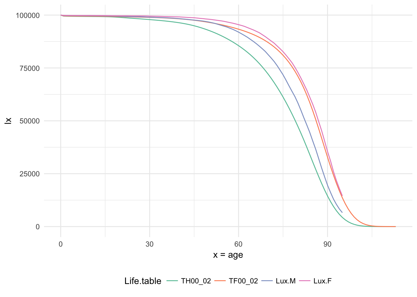
Unfortunately, the table stops at the age of 95. So according to the tables, Women in France and Luxembourg have similar \(l_x\) curves, but men in Luxembourg tend to live longer than those in France.
As expected, men in Luxembourg have a higher life expectancy at birth than those in France. The spread between men and women is therefore smaller (around 4.4 years).
Price of a whole life insurance contract
We now know how to compute the probability that a person aged \(x_0\) dies at the age of \(x\) which is \(\mathbb{P}[T=x|x_0] = \left[\frac{l_{x}-l_{x+1}}{l_{x_0}}\right]\). We can therefore compute the pure premium (without fees etc.) of a whole life insurance contract with a benefit of \(N\) monetary units (EUR, USD … you name it) payable at the end of the year of death : \[Premium(insurance)=\sum_{x=x_0}^\infty \left[ \mathbb{P}[T=x|x_0]\cdot N \cdot P(x-x_0+1)\right]\]
Let’s keep this simple and assume that there’s a constant interest rate \(i\), therefore \(P(x)=\frac{1}{(1+i)^x}\)
\[ \begin{aligned} Premium(insurance)&= N\cdot \sum_{x=x_0}^\infty \left[ \mathbb{P}[T=x|x_0]\cdot \frac{1}{(1+i)^{(x-x_0+1)}}\right] \\ &=N\cdot A_{x_0} \end{aligned} \]
\(A_{x_0}\) is called the actuarial present value of one unit of a whole life insurance contract for a person aged \(x_0\). Besides, there’s a nice function lifecontingencies::Axn that takes care of all these formulas.
International contracts
It’ll be interesting to see how much the same contract costs in different countries with different interest rates and different life tables. Let’s compare hypothetical contracts in Luxembourg, France, the United States and China and for the sake of simplicity, let’s consider the 10 year government bond yield as a proxy for the interest rates :
- Luxembourg : 0,40%
- France : 0,75%
- United States : 2,5%
- China : 4%
# Create a new unisex life table
## Luxembourg
B2307<-new("lifetable",
           x=as.numeric(gsub("[^0-9]","",B2307$age)),
           lx=B2307$Lux.F+B2307$Lux.M,
           name="B2307")
aB2307<-new("actuarialtable",
           x=B2307@x,
           lx=B2307@lx,
           interest=0.0040,
           name="aB2307")
## France
data("demoFrance")
THF<-new("lifetable",
         x=demoFrance$age,
         lx=demoFrance$TH00_02+demoFrance$TF00_02,
         name="THF00_02")

aTHF<-new("actuarialtable",
          x=THF@x,
          lx=THF@lx,
          interest=0.0075,
          name="aTHF00_02")
The chinese dataset here is defined by the probabilities to die \(q_x\), we must therefore convert it to a proper life table using lifecontingencies::probs2lifetable :
## China
data("demoChina")
CL1<-probs2lifetable(probs=demoChina$CL1,radix=1000,type="qx",name="CHINA CL1")
CL2<-probs2lifetable(probs=demoChina$CL2,radix=1000,type="qx",name="CHINA CL2")

aCL12<-new("actuarialtable",
          x=CL1@x,
          lx=CL1@lx+CL2@lx,
          interest=0.04,
          name="CL1+2")
## USA
data("soa08")
asoa08<-new("actuarialtable",
            x=soa08@x,
            lx=soa08@lx,
            interest=0.025,
            name="SOA08")

# -----------------------------------------

Ax<-foreach(x=0:95,.combine=rbind.data.frame)%do%{
  data.frame(age=x,
             LU=Axn(aB2307,x),
             FR=Axn(aTHF,x),
             CN=Axn(aCL12,x),
             US=Axn(asoa08,x)
             )
}
So if we plot the values of lifecontingencies::Axn we will get :
So to conclude, it is less expensive to buy a whole life insurance contract in China mostly due to the higher interest rates. But this assumes that insurance companies can only invest in local government bonds, something that is definitely not true. I’ll leave this for later in another article.
That’s it for today, thanks for reading and if you haven’t been able to pay a visit to your parents and/or grand-parents please take some time and do so.
Life is short, stay healthy and merry christmas :).
![]() END
END
